RandomSampling.ipynb

Discrete Probability Distribution

A discrete probability distribution is a probability distribution that can take on a countable number of values.In the case where the range of values is countably infinite, these values have to decline to zero fast enough for the probabilities to add up to 1. For example, if ${\displaystyle \operatorname {P} (X=n)={\tfrac {1}{2^{n}}}}$ for n = 1, 2, …, the sum of probabilities would be 1/2 + 1/4 + 1/8 + … = 1

Examples include the Poisson distribution, the Bernoulli distribution, and the binomial distribution.

When a sample (a set of observations) is drawn from a larger population, the sample points have an empirical distribution that is discrete, and which provides information about the population distribution.

Wikipedia

Probability Mass Function (PMF)

A probability mass function (PMF) is a function that gives the probability that a discrete random variable is exactly equal to some value. Sometimes it is also known as the discrete density function.

Cumulative Distribution Function (CDF)

A cumulative distribution function (CDF) of a random variable ${\displaystyle X}$ , or just distribution function of ${\displaystyle X}$, evaluated at ${\displaystyle x}$, is the probability that ${\displaystyle X}$ will take a value less than or equal to ${\displaystyle x}$.

Inverse distribution function (quantile function)

The quantile function, associated with a probability distribution of a random variable, specifies the value of the random variable such that the probability of the variable being less than or equal to that value equals the given probability. It is also called the percent-point function or inverse cumulative distribution function.

Wikipedia

Example

Here is an intuitive explanation:
Quora

P(Weak)=0.2 , P(Standard)=0.7, P(Strong) = 0.1

Continuous Probability Distribution

A continuous probability distribution is a probability distribution whose support is an uncountable set, such as an interval in the real line. They are uniquely characterized by a cumulative distribution function that can be used to calculate the probability for each subset of the support. There are many examples of continuous probability distributions: normal, uniform, chi-squared, and others.

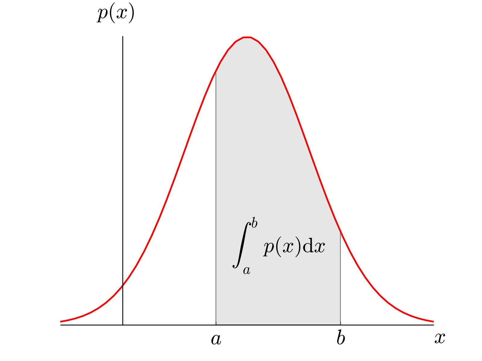
Probability Density Function (PDF)

A probability density function (PDF), or density of a continuous random variable, is a function whose value at any given sample (or point) in the sample space (the set of possible values taken by the random variable) can be interpreted as providing a relative likelihood that the value of the random variable would equal that sample. (Wikipedia)

Inverse Transform Sampling

Inverse transform sampling is a basic method for pseudo-random number sampling, i.e., for generating sample numbers at random from any probability distribution given its cumulative distribution function.

Example: Bernoulli Distribution

Theorem

Reference: Machine Learning - A Probabilistic Perspective, Kevin P. Murphy, Page 818

If $U\sim U(0,1)$ is a uniform random variable, then $F^{-1}(U)\sim F$

Proof:

$Pr(F^{-1}(U) \le x) = Pr(U \le F(x))$, applying F to both sides

$=F(x)$, because $Pr(U \le y)=y$

The first line follows since F is a monotonic function and the second line follows since U is uniform on the unit interval.

Example

The probability density function (pdf) of an exponential distribution is

${\displaystyle f(x;\lambda )={\begin{cases}\lambda e^{-\lambda x}&x\geq 0,\0&x<0.\end{cases}}}$

Here λ > 0 is the parameter of the distribution

The cumulative distribution function is given by

${\displaystyle F(x;\lambda )={\begin{cases}1-e^{-\lambda x}&x\geq 0,\0&x<0.\end{cases}}}$

The inverse cumulative function is

${\displaystyle F^{-1}(p)={\begin{cases} {\tfrac {-ln(1-p)}{\lambda}} &x\geq 0,\0&x<0.\end{cases}}}$

import numpy as np
                                     
lambda_1 = 2                                 
U=np.random.random(10000)            
X=-np.log(1-U)/lambda_1
np.mean(X)

0.49518234988983334

## Exercise.         

# is f(x) = 4*x on the interval [0,1] a density function? if not, what is the normalizing factor?
# What is the CDF?
# What is the inverse CDF?
# Use inverse sampling to estimate the expectation of the distribution

import numpy as np

# random numbers from a Bernoulli distribution (binary outcome) e.g., tossing a  coin heads/tails 10 times

 # 0----------p---1
                                 #.....
def bern(p):
  r = np.random.uniform(0,1)
  if r < p:
    return 1
  else:
    return 0

size = 10
for i in range(size):
  coin = bern(0.5)  # fair coin
  print(coin)

# off-the-shelf use of a library
from scipy.stats import bernoulli
size = 10
for i in range(size):
  coin = bernoulli.rvs(0.5)  # fair coin
  print(coin)

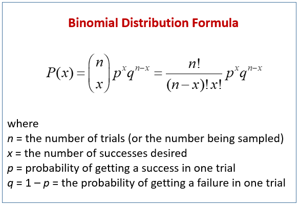
Example: Binomial Distribution

# Binomial distribution: binomial random variable counts the number of heads or positives or successes x in n repeated trials of a binomial experiment
# Example: simulation of the number of heads and tails by tossing a fair coin 10 times
def bern(p):
  r = np.random.uniform(0,1)
  if r < p:
    return 1
  else:
    return 0                     

size = 10
x = [0,1]
y = [0,0]

for i in range(size):
  index = bern(0.5)
  y[index] +=1

print(y)

[4, 6]

# Bernoulli as a special case of Binomial                     
                                                             
from scipy.stats import binom

size = 10
for i in range(size):
  coin = binom.rvs(1,0.5, size=1)  # fair coin       
  print(coin)

[0]
[0]
[0]
[0]
[1]
[0]
[1]
[1]
[1]
[0]

Example: Categorical Distribution

A categorical distribution (also called a generalized Bernoulli distribution, multinoulli distribution) is a discrete probability distribution that describes the possible results of a random variable that can take on one of K possible categories, with the probability of each category separately specified.(Wikipedia)

# Example: random outcomes of a die tossed 10 times

# 0-------p1--p1+p2------p1+p2+p3-------p1+p2+p3+p4----p1+p2+p3+p4+p5------1

def categ(p1,p2,p3,p4,p5,p6):
  r = np.random.uniform(0,1)
  if r < p1:
    return 1
  elif r < p1 + p2:
    return 2
  elif r < p1 + p2 + p3:
    return 3
  elif r < p1 + p2 + p3 + p4:
    return 4
  elif r < p1 + p2 + p3 + p4 + p5:
    return 5
  else: return 6

size = 10
for i in range(size):
  dice = categ(1/6,1/6, 1/6, 1/6, 1/6, 1/6)  # fair die
  print(dice)

Multinomial Distribution

# Multinomial distribution is the generalization of the binomial distribution when the categorical variable has more than two outcomes
# Example: Simulation of the number  of times each side of a fair die shows up if the die is tossed 10 times


y = [0,0,0,0,0,0,0] # initialize count to zero
size = 10

for i in range(size):
  dice = categ(1/6,1/6, 1/6, 1/6, 1/6, 1/6)
  y[dice] += 1
  
print(y[1:])

[0, 4, 2, 1, 1, 2]

Probability of multinomial distribution

$\frac{n!}{x_1!\cdots x_k!} p_1^{x_1} \cdots p_k^{x_k}$

Beta Distribution

The beta distribution is a family of continuous probability distributions defined on the interval [0, 1] parameterized by two positive shape parameters, denoted by α and β, that appear as exponents of the random variable and control the shape of the distribution. The generalization to multiple variables is called a Dirichlet distribution.

In Bayesian inference, the beta distribution is the conjugate prior probability distribution for the Bernoulli, binomial, negative binomial and geometric distributions. The beta distribution is a suitable model for the random behavior of percentages and proportions.

The probability density function (pdf) of the beta distribution, for 0 ≤ x ≤ 1, and shape parameters α, β > 0, is a power function of the variable x and of its reflection (1 − x) as follows:

${\displaystyle {\begin{aligned}f(x;\alpha ,\beta )&=\mathrm {constant} \cdot x^{\alpha -1}(1-x)^{\beta -1}\[3pt]&={\frac {x^{\alpha -1}(1-x)^{\beta -1}}{\displaystyle \int _{0}^{1}u^{\alpha -1}(1-u)^{\beta -1},du}}\[6pt]&={\frac {\Gamma (\alpha +\beta )}{\Gamma (\alpha )\Gamma (\beta )}},x^{\alpha -1}(1-x)^{\beta -1}\[6pt]&={\frac {1}{\mathrm {B} (\alpha ,\beta )}}x^{\alpha -1}(1-x)^{\beta -1}\end{aligned}}}$

where Γ(z) is the gamma function.

numpy.random.beta

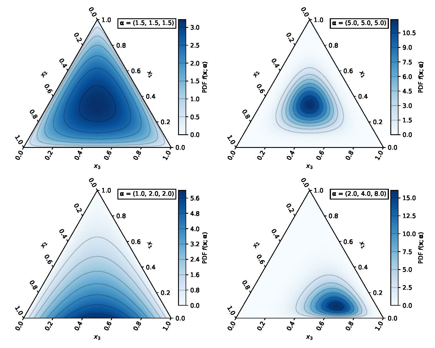
Dirichlet distribution

The Dirichlet distribution ${\displaystyle \operatorname {Dir} ({\boldsymbol {\alpha }})})$, is a family of continuous multivariate probability distributions parameterized by a vector ${\displaystyle {\boldsymbol {\alpha }}}$ of positive reals.

The Dirichlet distribution of order K ≥ 2 with parameters α1, …, αK > 0 has a probability density function given by

${\displaystyle f\left(x_{1},\ldots ,x_{K};\alpha {1},\ldots ,\alpha {K}\right)={\frac {1}{\mathrm {B} ({\boldsymbol {\alpha }})}}\prod {i=1}^{K}x{i}^{\alpha {i}-1}}$
where ${\displaystyle {x{k}}{k=1}^{k=K}}$ belong to the standard ${\displaystyle K-1}$ simplex, or in other words: ${\displaystyle \sum {i=1}^{K}x{i}=1{\mbox{ and }}x{i}\geq 0{\mbox{ for all }}i\in {1,\dots ,K}}$
The normalizing constant is the multivariate beta function, which can be expressed in terms of the gamma function:

${\displaystyle \mathrm {B} ({\boldsymbol {\alpha }})={\frac {\prod _{i=1}^{K}\Gamma (\alpha _{i})}{\Gamma \left(\sum _{i=1}^{K}\alpha _{i}\right)}},\qquad {\boldsymbol {\alpha }}=(\alpha _{1},\ldots ,\alpha _{K}).}$

np.random.dirichlet()

## Exercise
def categ3(p1,p2,p3):
  r = np.random.uniform(0,1)
  if r < p1:
    return 1
  elif r < p1 + p2:
    return 2
  else: return 3

d1 = np.random.dirichlet((1/100, 1/100, 1/100), 1) ## one die/dice

# Get 10 samples from d1 using the function categ3

d2 = np.random.dirichlet((100, 100, 100), 1)

# Get 10 samples from d2

# What is the difference between the samples from d1 and the samples from d2? 
# How is it related to the parameters of the dirichlet distribution?

Summary

Bernoulli has two outcomes, e.g., Success(1) with probaility p and Failure(0) with probabilty 1- p.

Binomial is about the count of number of successes in N trials. It is the sum of the Bernoullis (ones and zeros)

Categorical has more than two discrete outcomes with probabilities p1, p2, p3, ….

Multinomial is about the count of each category.

Bernoulli is a special case of categorical

Binomial is a special case of multinomial

Beta is a distribution on distributions (Bernoulli)

Dirichlet is a distribution on distributions (Categorical)

Beta is a special case of Dirichlet

Monte Carlo Methods

Monte Carlo methods, or Monte Carlo experiments, are a broad class of computational algorithms that rely on repeated random sampling to obtain numerical results. The underlying concept is to use randomness to solve problems that might be deterministic in principle.

Wikipedia

Example

For example, consider a quadrant (circular sector) inscribed in a unit square. Given that the ratio of their areas is
π
/
4
, the value of π can be approximated using a Monte Carlo method:

Draw a square, then inscribe a quadrant within it
Uniformly scatter a given number of points over the square
Count the number of points inside the quadrant, i.e. having a distance from the origin of less than 1

The ratio of the inside-count and the total-sample-count is an estimate of the ratio of the two areas,
π
/
4
. Multiply the result by 4 to estimate π.

import scipy

N = 100000
x_array = scipy.random.rand(N)
y_array = scipy.random.rand(N)
# generate N pseudorandom independent x and y-values on interval [0,1)
N_qtr_circle = sum(x_array ** 2 + y_array ** 2 < 1)
# Number of pts within the quarter circle x^2 + y^2 < 1 centered at the origin with radius r=1.
# True area of quarter circle is pi/4 and has N_qtr_circle points within it.
# True area of the square is 1 and has N points within it, hence we approximate pi with
pi_approx = 4 * float(N_qtr_circle) / N  # Typical values: 3.13756, 3.15156

Integration Issues

If an elementary function is differentiable, we can explicitly output its derivative (e.g., autodiff). Most integrable functions don’t have elementary antiderivative (e.g., $exp(-x^2)$ ). If the denominator in Bayes formula is an integral, it could be intractable

Monte Carlo approaches

$$E_p[f(x)] = \int f(x)p(x) dx \approx \frac{1}{n}\sum_{i} f(x_i)$$ $$x_i \sim p(x)$$

Rejection Sampling

If we don’t have CDF or cannot invert the CDF, then rejection sampling can be used, at least for lower dimensional spaces.

The algorithm (used by John von Neumann and dating back to Buffon and his needle) to obtain a sample from distribution ${\displaystyle X}$ with density ${\displaystyle f}$ using samples from distribution ${\displaystyle Y}$ with density ${\displaystyle g}$ is as follows:

Obtain a sample ${\displaystyle y}$ from distribution ${\displaystyle Y}$ and a sample ${\displaystyle u}$ from ${\displaystyle \mathrm {Unif} (0,1)}$ (the uniform distribution over the unit interval).
Check whether or not ${\textstyle u<f(y)/Mg(y)}$.
If this holds, accept ${\displaystyle y}$ as a sample drawn from ${\displaystyle f}$;
if not, reject the value of ${\displaystyle y}$ and return to the sampling step.
The algorithm will take an average of ${\displaystyle M}$ iterations to obtain a sample.

1
2
3

import numpy as np
import matplotlib.pyplot as plt
from scipy.stats import pearsonr

Example

Standard Normal Distribution $\tilde{p}(x)=e^{-x^{2}/2}$ without the normalizing denominator $Z={\frac {1}{\sqrt {2\pi }}}$

$p(x)={\frac {\tilde{p}(x)} {Z}}$

# We want to sample from this distribution, assuming the denominator is difficult to integrate
def p_tilde(x):
    return np.exp(-x**2/2)

# Here is a function (standard normal) easy to sample from. It gives us proposals
# For simplicity we chose p_tilde / Z as q
def q(x):
    return np.exp(-x**2/2)/np.sqrt(2*np.pi)

Target Distribution

M=10
denominator = np.sqrt(2*np.pi)

xvals = np.arange(-4,4,.1)
p_tilde_vals = [p_tilde(x) for x in xvals]
qvals = [M*p/denominator for p in p_tilde_vals]

plt.figure(figsize=(8,6))
plt.plot(xvals, p_tilde_vals)
plt.plot(xvals, qvals)
plt.legend(['p_tilde(x)', 'Mq(x)'], fontsize=15)
plt.xlabel('x', fontsize=15)
plt.ylabel('p_tilde(x)', fontsize=15)

Text(0, 0.5, 'p_tilde(x)')

denominator = np.sqrt(2*np.pi) # we know it this time but it could be an intractable integral
M=10

# proposals accepted
accepted = []


N = 1000000 # proposals

for _ in range(N):
    proposal = np.random.normal(0, 1)
    
    prob_accept = p_tilde(proposal) / (M*q(proposal))

    if np.random.random() < prob_accept:
        accepted.append(proposal)

1
2
3

print(np.mean(accepted))
print(np.var(accepted))
len(accepted)

0.002990957644427239
1.00051595341158





250428

1	(len(accepted) / N)*100

25.0428

Drawbacks

Rejection sampling can lead to a lot of unwanted samples being taken if the function being sampled is highly concentrated in a certain region, for example a function that has a spike at some location.

Large M –> few accepted

# Exercises:
## f(1) = 1, f(2) =2, f(3) = 3. Is f(x) a pmf? if not, what is the normalizing constant?


## is f(x) = 4*x on the interval [0,1] a density function? if not, what is the normalizing factor?
## choose g(x) = 1 as the proposal distribution
## Choose M=4 and M=10 to compare the wasted samples

# proposals accepted
accepted = []

M=10

N = 1000000 # proposals

for _ in range(N):
    proposal = np.random.random()
    
    prob_accept = 4*proposal / M*1 # y ~ q(y), prop_accept = 𝑓(𝑦)/𝑀𝑔(𝑦)
                                   # f(y) = 4*y, g(y)=1, M =10
    u = np.random.random()
    if u  < prob_accept:
        accepted.append(proposal)

1
2
3

print(np.mean(accepted))
print(np.var(accepted))
len(accepted)

0.6675852172604363
0.055471605869961006





199125

Importance Sampling

Importance sampling is a general technique for estimating properties of a particular distribution, while only having samples generated from a different distribution than the distribution of interest.

The basic idea of importance sampling is to sample the states from a different distribution to lower the variance of the estimation of E[X;P], or when sampling from P is difficult.

$$E_p[f(x)] = \int f(x)p(x) dx = \int f(x)\frac{p(x)}{q(x)}q(x) dx \approx \frac{1}{n} \sum_{i} f(x_i)\frac{p(x_i)}{q(x_i)}$$

$$ x_i \sim q(x)$$

Example

Let the dashed curve be standard normal N(0,1) with density p(x) and t_1 = 1.96, then p(t>t_1) = 0.025. Let f(x) = 1 if x > 1.96 and 0 otherwise

The solid curve is N(3,1) with density q(x).

# sampling from the p(x)
values = []
N = 1000000 # proposals

f = lambda x:x>1.96

## Sample from p
proposals = np.random.normal(loc=0,scale=1,size=N)
values = f(proposals)
print("average {} variance {}".format(np.mean(values), np.var(values)))

average 0.025196 variance 0.024561161584

# sampling from q(x) results less variance

from scipy import stats
f = lambda x:x>1.96
p = lambda x : stats.norm().pdf(x)
q = lambda x : stats.norm(loc=3,scale=1).pdf(x)

values = []
N = 1000000 # proposals

## Sample from q
proposals = np.random.normal(loc=3,scale=1,size=N)
    
values = f(proposals)*p(proposals)/q(proposals) 
    

print("average {} variance {}".format(np.mean(values), np.var(values)))

average 0.025031757655900575 variance 0.0022310917341863755

Confusion of multinomial vs categorical

In some fields such as natural language processing, categorical and multinomial distributions are synonymous and it is common to speak of a multinomial distribution when a categorical distribution is actually meant. This stems from the fact that it is sometimes convenient to express the outcome of a categorical distribution as a “1-of-K” vector (a vector with one element containing a 1 and all other elements containing a 0) rather than as an integer in the range ${\displaystyle 1\dots K}$; in this form, a categorical distribution is equivalent to a multinomial distribution over a single trial.

Reference

from scipy.stats import multinomial
#rv = multinomial(1, [1/6,1/6,1/6,1/6,1/6,1/6])
#rv.rvs(1)
multinomial.rvs(n=1, p=[1/6,1/6,1/6,1/6,1/6,1/6], size=1)

array([[0, 1, 0, 0, 0, 0]])

1
2
3

z=np.random.multinomial(1, [1/6.]*6, size=1)
print(np.argmax(z))
z

0





array([[1, 0, 0, 0, 0, 0]])

1 2	## We've defined the function categ() above categ(1/6,1/6, 1/6, 1/6, 1/6, 1/6)

1	np.random.choice( a=[1, 2, 3,4,5,6], size=1 , p=[1/6, 1/6, 1/6, 1/6,1/6, 1/6] )

array([4])

我见青山多妩媚，料青山见我应如是

01242022 Data606

Discrete Probability Distribution

Probability Mass Function (PMF)

Cumulative Distribution Function (CDF)

Inverse distribution function (quantile function)

Example

Continuous Probability Distribution

Probability Density Function (PDF)

Inverse Transform Sampling

Example: Bernoulli Distribution

Theorem

Example

Example: Binomial Distribution

Example: Categorical Distribution

Multinomial Distribution

$\frac{n!}{x_1!\cdots x_k!} p_1^{x_1} \cdots p_k^{x_k}$

Beta Distribution

numpy.random.beta

Dirichlet distribution

np.random.dirichlet()

Summary

Monte Carlo Methods

Example

Integration Issues

Monte Carlo approaches

Rejection Sampling

Example

Target Distribution

Drawbacks

Importance Sampling

Example

Confusion of multinomial vs categorical